![]()
![]()

![]()
![]()
![]()
![]()
metadpy is a Python implementation of standard Bayesian models of behavioural metacognition. It is aimed to provide simple yet powerful functions to compute standard indexes and metrics of signal detection theory (SDT) and metacognitive efficiency (meta-d’ and hierarchical meta-d’) [Fleming and Lau, 2014, Fleming, 2017]. The only input required is a data frame encoding task performances and confidence ratings at the trial level.
metadpy is written in Python 3. It uses Numpy, Scipy and Pandas for most of its operation, comprizing meta-d’ estimation using maximum likelihood estimation (MLE). The (Hierarchical) Bayesian modelling is implemented in Aesara (now renamed PyTensor for versions of pymc >5.0).
Installation#
The package can be installed using pip:
pip install metadpy
For most of the operations, the following packages are required:
Numpy (>=1.15)
Scipy (>=1.3.0)
Pandas (>=0.24)
Matplotlib (>=3.0.2)
Seaborn (>=0.9.0)
Bayesian models will require:
Why metadpy?#
metadpy stands for meta-d’ (meta-d prime) in Python. meta-d’ is a behavioural metric commonly used in consciousness and metacognition research. It is modelled to reflect metacognitive efficiency (i.e the relationship between subjective reports about performances and objective behaviour).
metadpy first aims to be the Python equivalent of the hMeta-d toolbox (Matlab and R). It tries to make these models available to a broader open-source ecosystem and to ease their use via cloud computing interfaces. One notable difference is that While the hMeta-d toolbox relies on JAGS for the Bayesian modelling of confidence data (see [4]) to analyse task performance and confidence ratings, metadpy is built on the top of pymc, and uses Hamiltonina Monte Carlo methods (NUTS).
For an extensive introduction to metadpy, you can navigate the following notebooks that are Python adaptations of the introduction to the hMeta-d toolbox written in Matlab by Olivia Faul for the Zurich Computational Psychiatry course.
Importing data#
Classical metacognition experiments contain two phases: task performance and confidence ratings. The task performance could for example be the ability to distinguish the presence of a dot on the screen. By relating trials where stimuli are present or absent and the response provided by the participant (Can you see the dot: yes/no), it is possible to obtain the accuracy. The confidence rating is proposed to the participant when the response is made and should reflect how certain the participant is about his/her judgement.
An ideal observer would always associate very high confidence ratings with correct task-I responses, and very low confidence ratings with an incorrect task-1 response, while a participant with a low metacognitive efficiency will have a more mixed response pattern.
A minimal metacognition dataset will therefore consist in a data frame populated with 5 columns:
Stimuli: Which of the two stimuli was presented [0 or 1].Response: The response made by the participant [0 or 1].Accuracy: Was the participant correct? [0 or 1].Confidence: The confidence level [can be continuous or discrete rating].ntrial: The trial number.
Due to the logical dependence between the Stimuli, Responses and Accuracy columns, in practice only two of those columns are necessary, the third being deduced from the others. Most of the functions in metadpy will accept DataFrames containing only two of these columns, and will automatically infer the missing information. Similarly, as the metacognition models described here does not incorporate the temporal dimension, the trial number is optional.
metadpy includes a simulation function that will let you create one such data frame for one or many participants and condition, controlling for a variety of parameters. Here, we will simulate 200 trials from participant having d=1 and c=0 (task performances) and a meta-d=1.5 (metacognitive sensibility). The confidence ratings were provided using a 1-to-4 rating scale.
from metadpy.utils import responseSimulation

simulation = responseSimulation(d=1, metad=2.0, c=0, nRatings=4, nTrials=5000)
simulation.head()
| Stimuli | Responses | Accuracy | Confidence | nTrial | Subject | |
|---|---|---|---|---|---|---|
| 0 | 1 | 0 | 0 | 2 | 0 | 0 |
| 1 | 1 | 1 | 1 | 1 | 1 | 0 |
| 2 | 1 | 1 | 1 | 1 | 2 | 0 |
| 3 | 1 | 1 | 1 | 3 | 3 | 0 |
| 4 | 1 | 1 | 1 | 3 | 4 | 0 |
from metadpy.utils import trials2counts

nR_S1, nR_S2 = trials2counts(
    data=simulation,
    stimuli="Stimuli",
    accuracy="Accuracy",
    confidence="Confidence",
    nRatings=4,
)
nR_S1, nR_S2
(array([656, 385, 385, 303, 432, 211,  87,  41]),
 array([ 44,  78, 213, 436, 320, 409, 397, 603]))
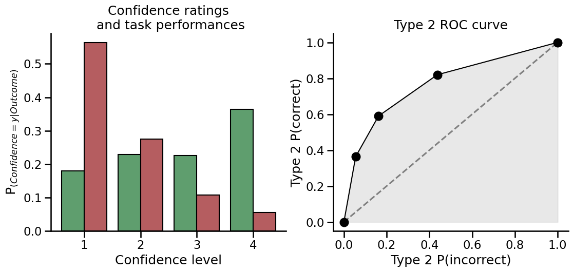
Data visualization#
You can easily visualize metacognition results using one of the plotting functions. Here, we will use the plot_confidence and the plot_roc functions to visualize the metacognitive performance of our participant.
import arviz as az
import matplotlib.pyplot as plt
import seaborn as sns
from metadpy.plotting import plot_confidence, plot_roc

sns.set_context("talk")
fig, axs = plt.subplots(1, 2, figsize=(13, 5))
plot_confidence(nR_S1, nR_S2, ax=axs[0])
plot_roc(nR_S1, nR_S2, ax=axs[1])
sns.despine()
Signal detection theory (SDT)#
All metadpy functions are registred as Pandas flavors (see pandas-flavor), which means that the functions can be called as a method from the result data frame. When using the default columns names (Stimuli, Response, Accuracy, Confidence), this significantly reduces the length of the function call, making your code more clean and readable.
simulation.criterion()
-0.0
simulation.dprime()
1.0007814013683562
simulation.rates()
(0.6916, 0.3084)
simulation.roc_auc(nRatings=4)
0.7665729304225586
simulation.scores()
(1729, 771, 771, 1729)
Estimating meta dprime using Maximum Likelyhood Estimates (MLE)#
from metadpy.mle import metad

results = metad(
    data=simulation,
    nRatings=4,
    stimuli="Stimuli",
    accuracy="Accuracy",
    confidence="Confidence",
    verbose=0,
)
results
| dprime | meta_d | m_ratio | m_diff | |
|---|---|---|---|---|
| 0 | 0.999911 | 1.867707 | 1.867873 | 0.867796 |
Estimating meta-d’ using Bayesian modeling#
Subject level#
from metadpy.bayesian import hmetad
model, trace = hmetad(
    data=simulation,
    nRatings=4,
    stimuli="Stimuli",
    accuracy="Accuracy",
    confidence="Confidence",
)
Auto-assigning NUTS sampler...
Initializing NUTS using jitter+adapt_diag...
Sequential sampling (4 chains in 1 job)
NUTS: [c1, d1, meta_d, cS1_hn, cS2_hn]
Sampling 4 chains for 1_000 tune and 1_000 draw iterations (4_000 + 4_000 draws total) took 68 seconds.
The rhat statistic is larger than 1.01 for some parameters. This indicates problems during sampling. See https://arxiv.org/abs/1903.08008 for details
The effective sample size per chain is smaller than 100 for some parameters. A higher number is needed for reliable rhat and ess computation. See https://arxiv.org/abs/1903.08008 for details
az.plot_trace(trace, var_names=["meta_d", "cS2", "cS1"]);
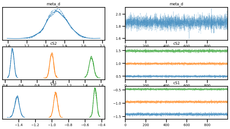
az.summary(trace, var_names=["meta_d", "cS2", "cS1"])
| mean | sd | hdi_3% | hdi_97% | mcse_mean | mcse_sd | ess_bulk | ess_tail | r_hat | |
|---|---|---|---|---|---|---|---|---|---|
| meta_d | 1.861 | 0.055 | 1.756 | 1.964 | 0.001 | 0.001 | 3333.0 | 3376.0 | 1.0 |
| cS2[0] | 0.492 | 0.020 | 0.456 | 0.528 | 0.000 | 0.000 | 4512.0 | 3308.0 | 1.0 |
| cS2[1] | 0.983 | 0.023 | 0.942 | 1.027 | 0.000 | 0.000 | 3573.0 | 3462.0 | 1.0 |
| cS2[2] | 1.479 | 0.028 | 1.426 | 1.532 | 0.000 | 0.000 | 3637.0 | 3117.0 | 1.0 |
| cS1[0] | -1.419 | 0.027 | -1.475 | -1.371 | 0.000 | 0.000 | 3354.0 | 3625.0 | 1.0 |
| cS1[1] | -0.954 | 0.023 | -0.995 | -0.910 | 0.000 | 0.000 | 3787.0 | 3508.0 | 1.0 |
| cS1[2] | -0.478 | 0.019 | -0.513 | -0.441 | 0.000 | 0.000 | 4608.0 | 3184.0 | 1.0 |