Fitting a psychometric function at the group level#
Author: Nicolas Legrand nicolas.legrand@cas.au.dk
import pytensor.tensor as pt
import arviz as az
import matplotlib.pyplot as plt
import numpy as np
import pandas as pd
import seaborn as sns
from scipy.stats import norm
import pymc as pm

sns.set_context('talk')
---------------------------------------------------------------------------
ModuleNotFoundError                       Traceback (most recent call last)
Cell In[1], line 1
----> 1 import pytensor.tensor as pt
      2 import arviz as az
      3 import matplotlib.pyplot as plt

ModuleNotFoundError: No module named 'pytensor'
In this example, we are going to fit a cummulative normal function to decision responses made during the Heart Rate Discrimination task. We will use the data from the HRD method paper [Legrand et al., 2022] and analyse the responses from all participants and infer group-level hyperpriors.
# Load data frame
psychophysics_df = pd.read_csv('https://github.com/embodied-computation-group/CardioceptionPaper/raw/main/data/Del2_merged.txt')
First, let’s filter this data frame so we only keep the interoceptive condition (Extero label).
this_df = psychophysics_df[psychophysics_df.Modality == 'Extero']
this_df.head()
| TrialType | Condition | Modality | StairCond | Decision | DecisionRT | Confidence | ConfidenceRT | Alpha | listenBPM | ... | EstimatedThreshold | EstimatedSlope | StartListening | StartDecision | ResponseMade | RatingStart | RatingEnds | endTrigger | HeartRateOutlier | Subject | |
|---|---|---|---|---|---|---|---|---|---|---|---|---|---|---|---|---|---|---|---|---|---|
| 1 | psi | Less | Extero | psi | Less | 2.216429 | 59.0 | 1.632995 | -0.5 | 78.0 | ... | 22.805550 | 12.549457 | 1.603353e+09 | 1.603354e+09 | 1.603354e+09 | 1.603354e+09 | 1.603354e+09 | 1.603354e+09 | False | sub_0019 |
| 3 | psiCatchTrial | Less | Extero | psiCatchTrial | Less | 1.449154 | 100.0 | 0.511938 | -30.0 | 82.0 | ... | NaN | NaN | 1.603354e+09 | 1.603354e+09 | 1.603354e+09 | 1.603354e+09 | 1.603354e+09 | 1.603354e+09 | False | sub_0019 |
| 6 | psi | More | Extero | psi | More | 1.182666 | 95.0 | 0.606786 | 22.5 | 69.0 | ... | 10.001882 | 12.884902 | 1.603354e+09 | 1.603354e+09 | 1.603354e+09 | 1.603354e+09 | 1.603354e+09 | 1.603354e+09 | False | sub_0019 |
| 10 | psi | More | Extero | psi | More | 1.848141 | 24.0 | 1.448969 | 10.5 | 62.0 | ... | 0.998384 | 13.044744 | 1.603354e+09 | 1.603354e+09 | 1.603354e+09 | 1.603354e+09 | 1.603354e+09 | 1.603354e+09 | False | sub_0019 |
| 11 | psiCatchTrial | More | Extero | psiCatchTrial | More | 1.349469 | 75.0 | 0.561820 | 10.0 | 72.0 | ... | NaN | NaN | 1.603354e+09 | 1.603354e+09 | 1.603354e+09 | 1.603354e+09 | 1.603354e+09 | 1.603354e+09 | False | sub_0019 |
5 rows × 25 columns
This data frame contain a large number of columns, but here we will be interested in the Alpha column (the intensity value) and the Decision column (the response made by the participant).
this_df = this_df[['Alpha', 'Decision', 'Subject']]
this_df.head()
| Alpha | Decision | Subject | |
|---|---|---|---|
| 1 | -0.5 | Less | sub_0019 |
| 3 | -30.0 | Less | sub_0019 |
| 6 | 22.5 | More | sub_0019 |
| 10 | 10.5 | More | sub_0019 |
| 11 | 10.0 | More | sub_0019 |
These two columns are enought for us to extract the 3 vectors of interest to fit a psychometric function:
The intensity vector, listing all the tested intensities values
The total number of trials for each tested intensity value
The number of “correct” response (here, when the decision == ‘More’).
Let’s take a look at the data. This function will plot the proportion of “Faster” responses depending on the intensity value of the trial stimuli (expressed in BPM). Here, the size of the circle represent the number of trials that were presented for each intensity values.
Model#
The model is defined as follows:
Where \(erf\) is the error functions, and \(\Phi\) is the cumulative normal function with threshold \(\alpha\) and slope \(\beta\).
We create our own cumulative normal distribution function here using pytensor.
def cumulative_normal(x, alpha, beta):
    # Cumulative distribution function for the standard normal distribution
    return 0.5 + 0.5 * pt.erf((x - alpha) / (beta * pt.sqrt(2)))
We preprocess the data to extract the intensity \(x\), the number or trials \(n\) and number of hit responses \(r\). We also create a vector sub_total containing the participants index (from 0 to \(n_{participants}\)).
nsubj = this_df.Subject.nunique()
x_total, n_total, r_total, sub_total = [], [], [], []

for i, sub in enumerate(this_df.Subject.unique()):

    sub_df = this_df[this_df.Subject==sub]

    x, n, r = np.zeros(163), np.zeros(163), np.zeros(163)

    for ii, intensity in enumerate(np.arange(-40.5, 41, 0.5)):
        x[ii] = intensity
        n[ii] = sum(sub_df.Alpha == intensity)
        r[ii] = sum((sub_df.Alpha == intensity) & (sub_df.Decision == "More"))

    # remove no responses trials
    validmask = n != 0
    xij, nij, rij = x[validmask], n[validmask], r[validmask]
    sub_vec = [i] * len(xij)

    x_total.extend(xij)
    n_total.extend(nij)
    r_total.extend(rij)
    sub_total.extend(sub_vec)
Create the model.
with pm.Model() as group_psychophysics:

    mu_alpha = pm.Uniform("mu_alpha", lower=-50, upper=50)
    sigma_alpha = pm.HalfNormal("sigma_alpha", sigma=100)

    mu_beta = pm.Uniform("mu_beta", lower=0, upper=100)
    sigma_beta = pm.HalfNormal("sigma_beta", sigma=100)

    alpha = pm.Normal("alpha", mu=mu_alpha, sigma=sigma_alpha, shape=nsubj)
    beta = pm.Normal("beta", mu=mu_beta, sigma=sigma_beta, shape=nsubj)

    thetaij = pm.Deterministic(
        "thetaij", cumulative_normal(x_total, alpha[sub_total], beta[sub_total])
    )

    rij_ = pm.Binomial("rij", p=thetaij, n=n_total, observed=r_total)
pm.model_to_graphviz(group_psychophysics)

Sampling.
with group_psychophysics:
    idata = pm.sample(chains=4, cores=4)
Auto-assigning NUTS sampler...
Initializing NUTS using jitter+adapt_diag...
Multiprocess sampling (4 chains in 4 jobs)
NUTS: [mu_alpha, sigma_alpha, mu_beta, sigma_beta, alpha, beta]
Sampling 4 chains for 1_000 tune and 1_000 draw iterations (4_000 + 4_000 draws total) took 93 seconds.
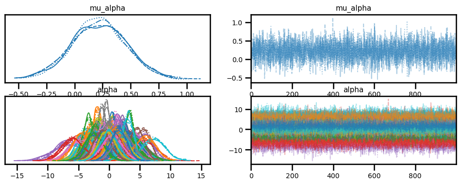
az.plot_trace(idata, var_names=["mu_alpha", "alpha"]);
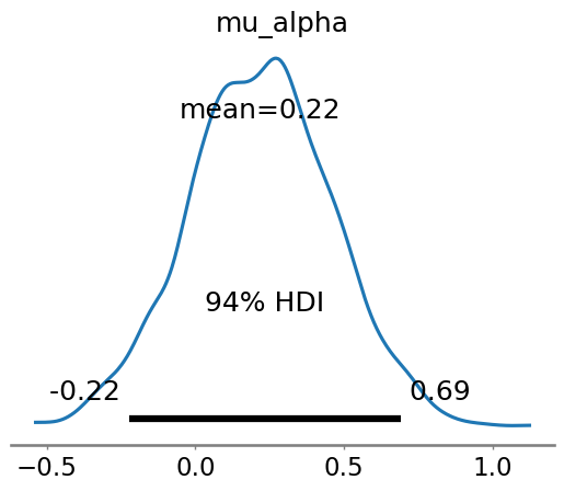
stats = az.summary(idata, var_names=["mu_alpha", "mu_beta"])
stats
| mean | sd | hdi_3% | hdi_97% | mcse_mean | mcse_sd | ess_bulk | ess_tail | r_hat | |
|---|---|---|---|---|---|---|---|---|---|
| mu_alpha | 0.218 | 0.241 | -0.224 | 0.691 | 0.004 | 0.003 | 4670.0 | 3227.0 | 1.0 |
| mu_beta | 7.926 | 0.233 | 7.516 | 8.370 | 0.004 | 0.003 | 2931.0 | 2961.0 | 1.0 |
az.plot_posterior(idata, var_names=["mu_alpha"])
<Axes: title={'center': 'mu_alpha'}>
Plotting#
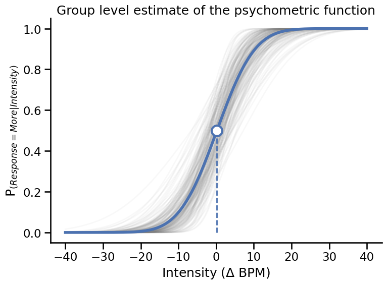
Extrace the individual parameters estimates.
alpha_samples = az.summary(idata, var_names=["alpha"])["mean"].values
beta_samples = az.summary(idata, var_names=["beta"])["mean"].values
fig, axs = plt.subplots(figsize=(8, 6))

# Draw some sample from the traces
for a, b in zip(alpha_samples, beta_samples):
    axs.plot(
        np.linspace(-40, 40, 500),
        (norm.cdf(np.linspace(-40, 40, 500), loc=a, scale=b)),
        color='gray', alpha=.05, linewidth=2
    )

# Plot psychometric function with average parameters
slope = az.summary(idata, var_names=["mu_beta"])['mean']['mu_beta']
threshold = az.summary(idata, var_names=["mu_alpha"])['mean']['mu_alpha']
axs.plot(np.linspace(-40, 40, 500),
        (norm.cdf(np.linspace(-40, 40, 500), loc=threshold, scale=slope)),
         color='#4c72b0', linewidth=4)

axs.plot([threshold, threshold], [0, .5], '--', color='#4c72b0', linewidth=2)
axs.plot(threshold, .5, 'o', color='w', markeredgecolor='#4c72b0',
         markersize=15, markeredgewidth=3)

plt.ylabel('P$_{(Response = More|Intensity)}$')
plt.xlabel('Intensity ($\Delta$ BPM)')
plt.title('Group level estimate of the psychometric function')
plt.tight_layout()
sns.despine()
System configuration#
%load_ext watermark
%watermark -n -u -v -iv -w -p pymc,arviz,pytensor
Last updated: Wed Jun 28 2023

Python implementation: CPython
Python version       : 3.11.4
IPython version      : 8.14.0

pymc    : 5.5.0
arviz   : 0.15.1
pytensor: 2.12.3

numpy     : 1.24.4
matplotlib: 3.7.1
arviz     : 0.15.1
seaborn   : 0.12.2
pymc      : 5.5.0
pandas    : 2.0.2
pytensor  : 2.12.3

Watermark: 2.4.2