Detecting and correcting artefacts in RR time series

This example describes artefacts correction in RR time series.

The function correct_rr() automatically detect artefacts using the method proposed by Lipponen & Tarvainen (2019) 1. Shorts, extra, long, missed and ectopic beats are corrected using either inserion/delection of RR intervals or interpolation of the RR time series, and the detection procedure is run again using cleaned intervals. Importantly, when using this method the signal length can be altered after the interpolation, introducing misalignement with eg. triggers from the experiment. For this reason, it is only recommended to use it in the context of “bloc design” study, when heart rate variability is measured for a given time interval (usually > 5 minutes).

# Author: Nicolas Legrand <nicolas.legrand@cfin.au.dk>
# Licence: GPL v3

import matplotlib.pyplot as plt
import numpy as np
import pandas as pd
import seaborn as sns

from systole import import_dataset1
from systole.correction import correct_rr
from systole.detection import ecg_peaks
from systole.hrv import frequency_domain
from systole.plots import plot_frequency, plot_rr
from systole.utils import input_conversion

ecg_df = import_dataset1(modalities=['ECG', 'Stim'])

  0%|          | 0/2 [00:00<?, ?it/s]
Downloading ECG channel:   0%|          | 0/2 [00:00<?, ?it/s]
Downloading ECG channel:  50%|█████     | 1/2 [00:00<00:00,  2.67it/s]
Downloading Stim channel:  50%|█████     | 1/2 [00:00<00:00,  2.67it/s]
Downloading Stim channel: 100%|██████████| 2/2 [00:00<00:00,  2.18it/s]
Downloading Stim channel: 100%|██████████| 2/2 [00:00<00:00,  2.24it/s]

signal, peaks = ecg_peaks(ecg_df.ecg, method='pan-tompkins', sfreq=1000)

rr_ms = input_conversion(peaks, input_type="peaks", output_type="rr_ms")

are using Matplotlib as plotting backend.

plot_rr(rr_ms, input_type='rr_ms', figsize=(13, 5))

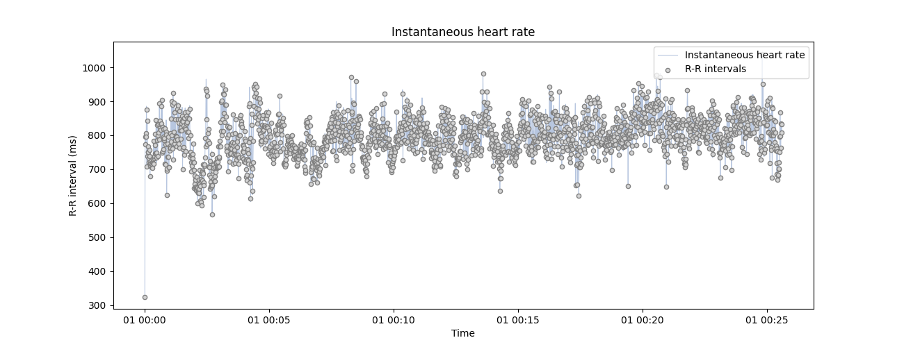
<Axes: title={'center': 'Instantaneous heart rate'}, xlabel='Time', ylabel='R-R interval (ms)'>

peaks and extra peaks by manually increasing or decreasing the length of some RR intervals.

np.random.seed(123)  # For result reproductibility

corrupted_rr = rr_ms.copy()  # Create a new RR intervals vector

# Randomly select 50 intervals in the time series and multiply them by 2 (missed peaks)
corrupted_rr[np.random.choice(len(corrupted_rr), 50)] *= 2

# Randomly select 50 intervals in the time series and divide them by 3 (extra peaks)
corrupted_rr[np.random.choice(len(corrupted_rr), 50)] /= 3

using show_artefacts=True so the artefacts detection runs automatically and shows in the plot.

plot_rr(
    corrupted_rr, input_type='rr_ms', show_artefacts=True, line=False, figsize=(13, 5)
    )
plt.show()

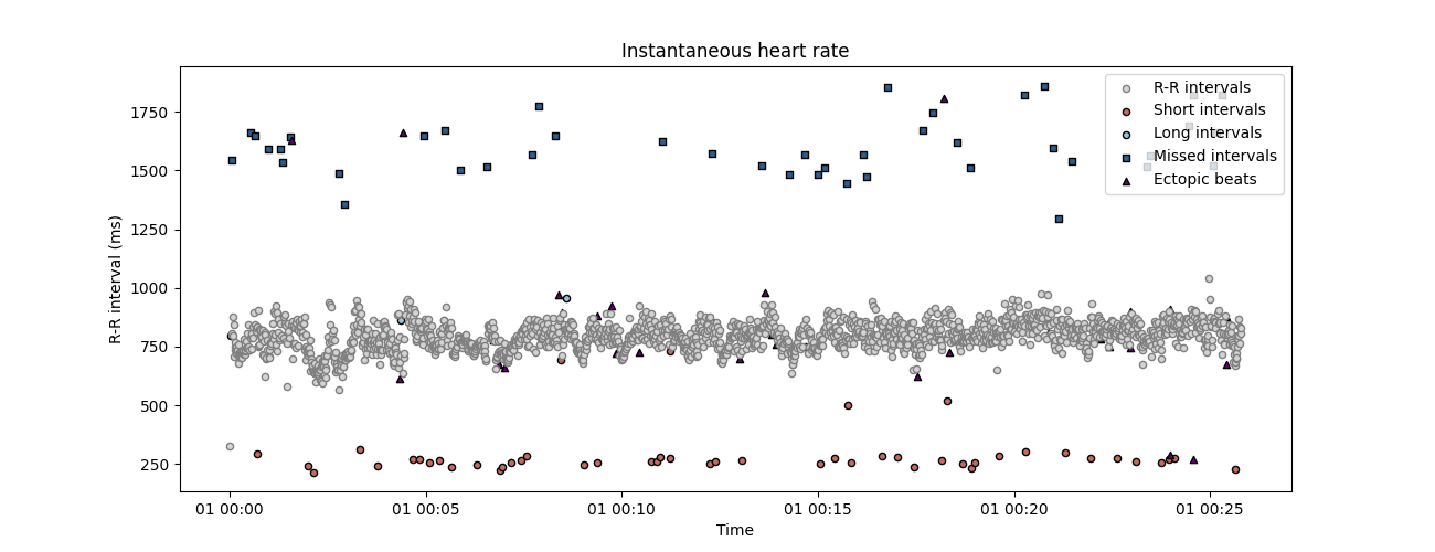
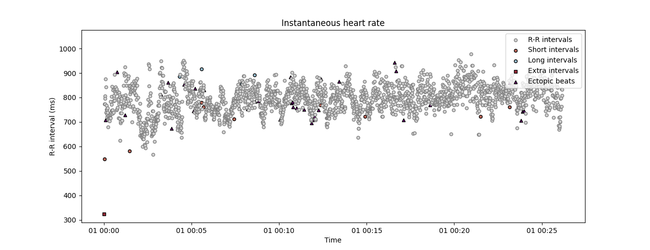
and short RR intervals and they are later correctly detected. We can now apply the RR time series correction method. This function will automatically detect possible artefacts in the RR intervals and reconstruct the most probable value using time series interpolation. The number of iteration is set to 2 by default, we add it here for clarity.

corrected_rr, _ = correct_rr(corrupted_rr)

Cleaning the RR interval time series.
... correcting 43 missed interval(s).
... correcting 34 ectopic interval(s).
... correcting 47 short interval(s).
... correcting 3 long interval(s).

plot_rr(corrected_rr, input_type='rr_ms', show_artefacts=True,
        line=False, figsize=(13, 5))
plt.show()

This does not means that the new values match exactly the RR intervals, and the new corrected time series will always slightly differs from the original one. However, we can estimate how large this difference is by comparing the true, corrupted and corrected time series a posteriori. Here, instead of comparing the time series side by side, we can have a look at some HRV metrics that are known to be affected by RR artefacts, like the high frequency HRV.

_, axs = plt.subplots(1, 3, figsize=(13, 5), sharey=True)
for i, rr, lab in zip(range(3),
                 [rr_ms, corrupted_rr, corrected_rr],
                 ["Original", "Corrupted", "Corrected"]):
    plot_frequency(rr, input_type="rr_ms", ax=axs[i])
    axs[i].set_title(lab)

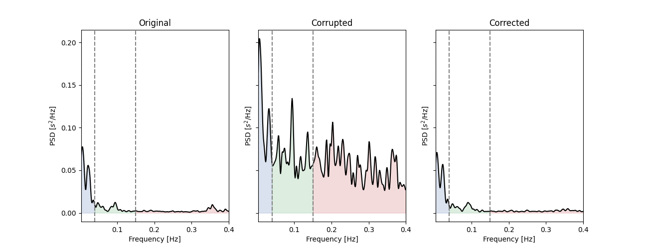
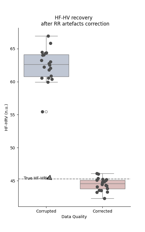
similar frequency dynamic. To get a more quantitative view of this resultm e can simply repeat this process of RR corruption-correction many time and check the HF-HRV parameters estimated at each steps.

# Clean the RR time series before simulation
corrected_rr, _ = correct_rr(rr_ms.copy())

simulation_df = pd.DataFrame([])
for i in range(20):

    # Measure HF-HRV for corrupted RR intervals time series
    corrupted_rr = corrected_rr.copy()
    corrupted_rr[np.random.choice(len(corrupted_rr), 50)] *= 2
    corrupted_rr[np.random.choice(len(corrupted_rr), 50)] /= 3
    corrupted_hrv = frequency_domain(corrupted_rr, input_type="rr_ms")
    corrupted_hf = corrupted_hrv[corrupted_hrv.Metric == "hf_power_nu"].Values.iloc[0]

    # Measure HF-HRV for corrected RR intervals time series
    corrected, _ = correct_rr(corrupted_rr, verbose=False)
    corrected_hrv = frequency_domain(corrected, input_type="rr_ms")
    corrected_hf = corrected_hrv[corrected_hrv.Metric == "hf_power_nu"].Values.iloc[0]

    simulation_df = pd.concat(
        [
            simulation_df,
            pd.DataFrame(
                {"HF-HRV (n.u.)": [corrupted_hf, corrected_hf],
                 "Data Quality": ["Corrupted", "Corrected"]
                }
                )
        ]
    )

initial_hrv = frequency_domain(corrected_rr, input_type="rr_ms")
initial_hf = initial_hrv[initial_hrv.Metric == "hf_power_nu"].Values.iloc[0]

Cleaning the RR interval time series.
... correcting 65 ectopic interval(s).
... correcting 4 short interval(s).
... correcting 4 long interval(s).

plt.figure(figsize=(5, 8))
sns.boxplot(data=simulation_df, x="Data Quality", y="HF-HRV (n.u.)", palette="vlag")
sns.stripplot(data=simulation_df, x="Data Quality", y="HF-HRV (n.u.)",
              size=8, color=".3", linewidth=0)
plt.axhline(y=initial_hf, linestyle="--", color="gray")
plt.title("HF-HV recovery \n after RR artefacts correction")
plt.annotate("True HF-HRV", xy=(0, initial_hf), xytext=(-0.4, initial_hf - 0.05),
             arrowprops = dict(facecolor ='grey', shrink = 0.05))
sns.despine()
plt.show()

/home/runner/work/systole/systole/docs/source/examples/Artefacts/plot_RRCorrection.py:135: FutureWarning:

Passing `palette` without assigning `hue` is deprecated and will be removed in v0.14.0. Assign the `x` variable to `hue` and set `legend=False` for the same effect.

  sns.boxplot(data=simulation_df, x="Data Quality", y="HF-HRV (n.u.)", palette="vlag")

affected by the presence of simulated artefacts, the proposed correction methods allows to recover the true parameter with some precision.

References

1

Lipponen, J. A., & Tarvainen, M. P. (2019). A robust algorithm for heart rate variability time series artefact correction using novel beat classification. Journal of Medical Engineering & Technology, 43(3), 173–181. https://doi.org/10.1080/03091902.2019.1640306