Detecting and correcting artefacts#
Author: Nicolas Legrand nicolas.legrand@cfin.au.dk
Show code cell source
%%capture
import sys
if 'google.colab' in sys.modules:
    ! pip install systole
import matplotlib.pyplot as plt
import numpy as np
import seaborn as sns
from bokeh.io import output_notebook
from bokeh.plotting import show
from systole import import_dataset1
from systole.correction import correct_peaks, correct_rr
from systole.detection import ecg_peaks
from systole.plots import (plot_evoked, plot_frequency, plot_raw, plot_rr,
                           plot_subspaces)
from systole.utils import input_conversion

output_notebook()

sns.set_context('talk')
In this notebook, we introduce two methods for artefact detection and correction based on the peaks vector or the RR time series, respectively. ECG and PPG recording and the resulting R-R interval time series can be noisy, either due to artefacts in the signal or invalid peak detection. Common sources of signal artefacts in the signal are participant movements or sub-optimal recording setup (e.g., power line noise). These artefacts can be attenuated or removed by using appropriate filtering approaches, or ultimately by checking the recorded signal and manually correcting the time series. However, even when using valid ECG and PPG recording, the heart can adapt its frequency in a way that can appear unlikely considering the RR intervals distributions and dynamics. Artefact detection and correction methods try to dissociate true artefacts induced by low-quality signals and irregular heart rate frequency.
# Import ECg recording
ecg_df = import_dataset1(modalities=['ECG', "Stim"], disable=True)

# Select the first minute of recording
signal = ecg_df.ecg.to_numpy()

# R peaks detection
signal, peaks = ecg_peaks(signal=signal, method='sleepecg', sfreq=1000)

# Convert peaks vector to RR time series
rr = input_conversion(peaks, input_type='peaks', output_type='rr_ms')
Following [Lipponen and Tarvainen, 2019], we distinguish between three kinds of irregular RR intervals, aka inter-beat intervals (IBIs):
Missing R peaks / long beats. This artefact corresponds to an interval that is longer than expected. The missed peaks suggest that an actual heartbeat was not correctly detected.
Extra R peaks or short beats. This artefact corresponds to an interval that is shorter than expected. The extra peak suggests that an R wave is erroneously detected.
Ectopic beats forming negative-positive-negative (NPN) or positive-negative-positive (PNP) segments.
Heart rate variability metrics are highly sensitive to such R-R artefacts, it is therefore critical to perform a careful artefact detection and correction procedure before extracting the heart rate variability metrics.
Artefacts detection#
Systole implements artefact detection based on adaptive thresholding of first and second derivatives of the R-R interval time series (see [Lipponen and Tarvainen, 2019] for a description of the method). One way to visualize the distribution of regular and irregular intervals is to use the transformation plotted below, which can be used to detect ectopic beats and long/short intervals. In the figure, the grey areas indicate the range of unlikely values considering each artefacts subtype. The intervals that are falling in these areas will be labelled as irregular.
show(
    plot_subspaces(rr, input_type='rr_ms', backend='bokeh', figsize=400)
)
It is also possible to automatically propagate this information to the R-R interval time series plot itself so we can visualize exactly where the artefacts are located in the signal. You can achieve this behavior by setting show_artefacts to True.
show(
    plot_raw(signal, backend='bokeh', show_artefacts=True, show_heart_rate=True, figsize=300)
)
BokehDeprecationWarning: CDSView.source is no longer needed, and is now ignored. In a future release, passing source will result an error.
BokehDeprecationWarning: CDSView.filters was deprecated in bokeh 3.0. Use CDSView.filter instead.
BokehDeprecationWarning: CDSView.source is no longer needed, and is now ignored. In a future release, passing source will result an error.
BokehDeprecationWarning: CDSView.filters was deprecated in bokeh 3.0. Use CDSView.filter instead.
BokehDeprecationWarning: CDSView.source is no longer needed, and is now ignored. In a future release, passing source will result an error.
BokehDeprecationWarning: CDSView.filters was deprecated in bokeh 3.0. Use CDSView.filter instead.
As we can see in the figure above, the majority of detected R peaks are correctly localized, and the RR interval time series for the most part well estimated. There are few notable exceptions however, including extra R waves and the erroneous detection of artefacts around these areas. Note that, because the artefact detection method uses different orders of the derivative to estimate the regularity of the interval, the presence of actual artefacts can distort this process and induce false-positive around the true artefacts. That is why data cleaning should proceed first with the correction of the more salient divergences (i.e., missed and extra peaks) before correcting the less salient ones (i.e., long and short peaks). The correction of ectopic beats is more nuanced and depends on the exact experimental context (see below).
Artefact correction#
Well-calibrated automated R-R intervals artefact detection can often find issues that mere visual inspection of raw data may miss. Corrected these artefacts can in turn help to estimate heart rate variability more accurately, limiting the occurence of erroneous conclusions (i.e., type-I and type-II errors). The appropriate correction method depends on the nature of the artefact. It can be something that you might want to code yourself or correct manually by placing or removing peaks in the raw signal. It can also be a more automated process - regardless of the choice of automatic or manual correction, the correction procedure should be documented in a transparent and reproducible manner.
Systole provides two correction methods (correct_rr and correct_peaks). The choice between these two methods mostly depends on the level of signal preservation we want to achieve after correction: do we want to recreate a new RR time series that does not contains irregular intervals, or do we want a better detection of the R peaks themselves?
correct_rr: will operate on the RR time series directly and will return another time series that can have a different timing (as the cumulative sum of the R interval will change).
correct_peaks: will operate on the peaks vector directly. The number of peaks (and therefore the RR intervals) can vary, but the timing will remain constant.
The approach is often prefered for heart rate variability studies. In this case, long recordings of the heart rate (>5 minutes) are used and a robust estimate of some HRV metrics is estimated. Because we do not want this estimate to be contaminated by extreme RR intervals or even smaller deviations, those intervals are corrected by interpolation to make the time series as standard as possible, sacrificing the temporal precision of the heartbeat occurrence.
The second method is more appropriate when the temporal precision of the heartbeat detection is relevant (this can concern heartbeat evoked potentials or instantaneous heart rate variability when it is time-locked to some specific stimuli, see tutorial 5). In this case, instead of blind interpolation, the raw signal time series can be used to re-estimate the peaks.
Correcting atefacts in RR time series#
Note
See also the example Detecting and correcting artefacts in RR time series in the example gallery.
To illustrate how the correct_rr method can remove RR artefacts, we will use the RR interval time series extracted from the previous recording.
# Convert the peaks vector into RR intervals time series.
rr_ms = input_conversion(peaks, input_type="peaks", output_type="rr_ms")
Creating artefacts#
For now, this time series it not severely artefacted. But we can easily simulate missed peaks and extra peaks by manually increasing or decreasing the length of some RR intervals.
np.random.seed(123)  # For result reproducibility

corrupted_rr = rr_ms.copy()  # Create a new RR intervals vector

# Randomly select 50 intervals in the time series and multiply them by 2 (missed peaks)
corrupted_rr[np.random.choice(len(corrupted_rr), 50)] *= 2

# Randomly select 50 intervals in the time series and divide them by 3 (missed peaks)
corrupted_rr[np.random.choice(len(corrupted_rr), 50)] /= 3
Lets see if the artefact we created are correctly detected. Note that here, we are using show_artefacts=True so the artefacts detection runs automatically and shows in the plot.
show(
    plot_rr(corrupted_rr, input_type="rr_ms", show_artefacts=True,  line=False, backend="bokeh", figsize=300)
)
BokehDeprecationWarning: CDSView.source is no longer needed, and is now ignored. In a future release, passing source will result an error.
BokehDeprecationWarning: CDSView.filters was deprecated in bokeh 3.0. Use CDSView.filter instead.
BokehDeprecationWarning: CDSView.source is no longer needed, and is now ignored. In a future release, passing source will result an error.
BokehDeprecationWarning: CDSView.filters was deprecated in bokeh 3.0. Use CDSView.filter instead.
BokehDeprecationWarning: CDSView.source is no longer needed, and is now ignored. In a future release, passing source will result an error.
BokehDeprecationWarning: CDSView.filters was deprecated in bokeh 3.0. Use CDSView.filter instead.
BokehDeprecationWarning: CDSView.source is no longer needed, and is now ignored. In a future release, passing source will result an error.
BokehDeprecationWarning: CDSView.filters was deprecated in bokeh 3.0. Use CDSView.filter instead.
Correcting artefacts#
The artefacts simulation seems to work fine so far. We have created abnormal long and short RR intervals and they are later correctly detected. We can now apply the RR time series correction method. This function will automatically detect possible artefacts in the RR intervals and reconstruct the most probable value using time series interpolation.
corrected_rr, _ = correct_rr(corrupted_rr)
Cleaning the RR interval time series.
... correcting 43 missed interval(s).
... correcting 12 ectopic interval(s).
... correcting 49 short interval(s).
... correcting 4 long interval(s).
Let’s now have a look at the corrected RR time series.
show(
    plot_rr(
        corrected_rr, input_type='rr_ms', backend="bokeh", show_artefacts=True,
        line=False, figsize=300
        )
)
BokehDeprecationWarning: CDSView.source is no longer needed, and is now ignored. In a future release, passing source will result an error.
BokehDeprecationWarning: CDSView.filters was deprecated in bokeh 3.0. Use CDSView.filter instead.
BokehDeprecationWarning: CDSView.source is no longer needed, and is now ignored. In a future release, passing source will result an error.
BokehDeprecationWarning: CDSView.filters was deprecated in bokeh 3.0. Use CDSView.filter instead.
BokehDeprecationWarning: CDSView.source is no longer needed, and is now ignored. In a future release, passing source will result an error.
BokehDeprecationWarning: CDSView.filters was deprecated in bokeh 3.0. Use CDSView.filter instead.
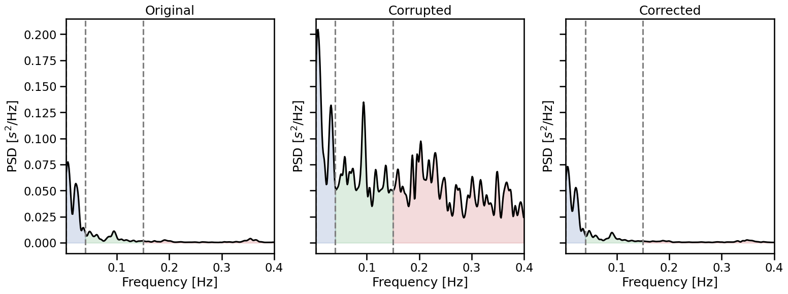
Visualization of the correction quality#
We can see that after two iterations, nearly all of of the artefacts have been corrected. This does not means that the new values match exactly the RR intervals, and the new corrected time series will always slightly differ from the original one. However, we can estimate how large this difference is by comparing the true, corrupted and corrected time series a posteriori. Here, instead of comparing the time series side by side, we can inspect HRV metrics that are known to be affected by RR artefacts, like the high frequency HRV.
_, axs = plt.subplots(1, 3, figsize=(18, 6), sharey=True)
for i, rr, lab in zip(range(3),
                 [rr_ms, corrupted_rr, corrected_rr],
                 ["Original", "Corrupted", "Corrected"]):
    plot_frequency(rr, input_type="rr_ms", ax=axs[i])
    axs[i].set_title(lab)
Correcting artefacts in peaks vector#
Note
See also the exxample Detecting and correcting artefacts in RR time series in the example gallery.
Here, we are going to use the same recording, but this time correcting directly the peaks vector to demonstrate the use of correct_peaks.
Creating artefacts#
np.random.seed(123)  # For result reproductibility

corrupted_peaks = peaks.copy()  # Create a new RR intervals vector

# Randomly select 50 peaks in the peask vector and set it to 0 (missed peaks)
corrupted_peaks[np.random.choice(np.where(corrupted_peaks)[0], 50)] = 0

# Randomly add 50 intervals in the peaks vector (extra peaks)
corrupted_peaks[np.random.choice(len(corrupted_peaks), 50)] = 1
show(
    plot_rr(corrupted_peaks, input_type="peaks", show_artefacts=True,  line=False, backend="bokeh", figsize=300)
)
BokehDeprecationWarning: CDSView.source is no longer needed, and is now ignored. In a future release, passing source will result an error.
BokehDeprecationWarning: CDSView.filters was deprecated in bokeh 3.0. Use CDSView.filter instead.
BokehDeprecationWarning: CDSView.source is no longer needed, and is now ignored. In a future release, passing source will result an error.
BokehDeprecationWarning: CDSView.filters was deprecated in bokeh 3.0. Use CDSView.filter instead.
BokehDeprecationWarning: CDSView.source is no longer needed, and is now ignored. In a future release, passing source will result an error.
BokehDeprecationWarning: CDSView.filters was deprecated in bokeh 3.0. Use CDSView.filter instead.
BokehDeprecationWarning: CDSView.source is no longer needed, and is now ignored. In a future release, passing source will result an error.
BokehDeprecationWarning: CDSView.filters was deprecated in bokeh 3.0. Use CDSView.filter instead.
BokehDeprecationWarning: CDSView.source is no longer needed, and is now ignored. In a future release, passing source will result an error.
BokehDeprecationWarning: CDSView.filters was deprecated in bokeh 3.0. Use CDSView.filter instead.
Correcting artefacts#
Again, the simulated artefact detection has worked as intended. We can now apply the peak correction method. This function will automatically detect possible artefacts in the peak vector and reconstruct the most coherent values using time series interpolation. The number of iteration is set to 2 by default, we add it here for clarity. Here, the correct_peaks function only correct for extra and missed peaks. This feature is intentional and reflects the notion that only artefacts in R peaks detection should be corrected, but “true” intervals that are anomaly shorter or longer should not be corrected.
peaks_correction = correct_peaks(corrupted_peaks)
Cleaning the peaks vector using 1 iterations.
 - Iteration 1 -
... correcting 45 extra peak(s).
... correcting 44 missed peak(s).
show(
    plot_rr(peaks_correction["clean_peaks"], input_type="peaks", show_artefacts=True,  line=False, backend="bokeh", figsize=300)
)
BokehDeprecationWarning: CDSView.source is no longer needed, and is now ignored. In a future release, passing source will result an error.
BokehDeprecationWarning: CDSView.filters was deprecated in bokeh 3.0. Use CDSView.filter instead.
BokehDeprecationWarning: CDSView.source is no longer needed, and is now ignored. In a future release, passing source will result an error.
BokehDeprecationWarning: CDSView.filters was deprecated in bokeh 3.0. Use CDSView.filter instead.
BokehDeprecationWarning: CDSView.source is no longer needed, and is now ignored. In a future release, passing source will result an error.
BokehDeprecationWarning: CDSView.filters was deprecated in bokeh 3.0. Use CDSView.filter instead.
BokehDeprecationWarning: CDSView.source is no longer needed, and is now ignored. In a future release, passing source will result an error.
BokehDeprecationWarning: CDSView.filters was deprecated in bokeh 3.0. Use CDSView.filter instead.
BokehDeprecationWarning: CDSView.source is no longer needed, and is now ignored. In a future release, passing source will result an error.
BokehDeprecationWarning: CDSView.filters was deprecated in bokeh 3.0. Use CDSView.filter instead.
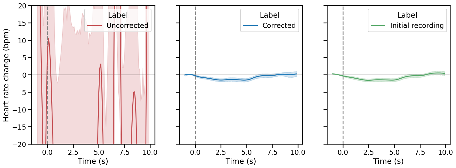
Visualization of the correction quality#
As previously mentioned, this method is more appropriate in the context of event-related analysis, where the evolution of the instantaneous heart rate is assessed after some experimental manipulation (see Tutorial 5). One way to control for the quality of the artefact correction is to compare the evoked responses measured under corrupted, corrected and baseline recording. Here, we will use the plot_evoked function, which simply take the indexes of events as input together with the recording (here the peaks vector), and produce the evoked plots.
# Merge the two conditions together.
# The events of interest are all data points that are not 0.
triggers_idx = [np.where(ecg_df.stim.to_numpy() != 0)[0]]
_, axs = plt.subplots(1, 3, figsize=(18, 6), sharey=True)
plot_evoked(rr=corrupted_peaks, triggers_idx=triggers_idx, ci=68,
            input_type="peaks", decim=100, apply_baseline=(-1.0, 0.0), figsize=(8, 8),
            labels="Uncorrected", palette=["#c44e52"], ax=axs[0])
plot_evoked(rr=peaks_correction["clean_peaks"], triggers_idx=triggers_idx, ci=68,
            input_type="peaks", decim=100, apply_baseline=(-1.0, 0.0), figsize=(8, 8),
            labels="Corrected", ax=axs[1])
plot_evoked(rr=peaks, triggers_idx=triggers_idx, ci=68, palette=["#55a868"],
            input_type="peaks", decim=100, apply_baseline=(-1.0, 0.0), figsize=(8, 8),
            labels="Initial recording", ax=axs[2])
plt.ylim(-20, 20);
/opt/hostedtoolcache/Python/3.9.18/x64/lib/python3.9/site-packages/systole/plots/backends/matplotlib/plot_evoked.py:70: FutureWarning:

The `ci` parameter is deprecated. Use `errorbar=('ci', 68)` for the same effect.

  sns.lineplot(data=epoch_df, x="Time", y="heart_rate", hue="Label", ax=ax, **kwargs)
This concludes the tutorial on using Systole to detect and correct more complex artefacts. In the next tutorial we will introduce more advanced signal processing techniques for estimating low and high-frequency heart-rate variability.
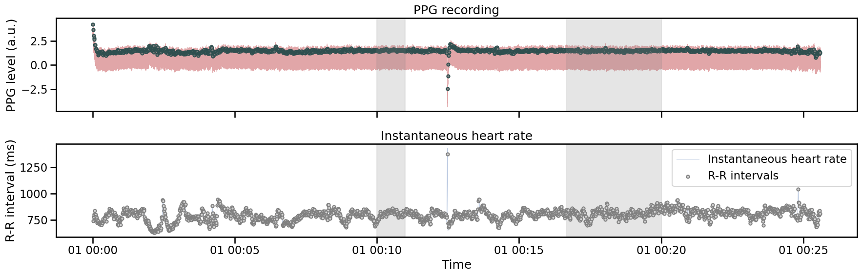
Handling bad segments in the physiological recording#
In some situations, the physiological recording will contain one or many invalid segments in the middle of the recording. If those segments are longer than a few seconds, the peaks cannot be reliably estimated and most of the heart rate variability metrics will not be valid, even after applying the correction listed above. We can consider a bad segment when 3 or more consecutive beats cannot be detected, and using interpolation will cause more harm in this context. Such bad segments can be manually labelled using the Viewer (see {the section on how to use the Viewer}viewer).
Most functions will let you provide bad_segments arguments and will try to handle the data accordingly. Using the same ECG recording as in the previous examples, we can annotate the raw plot by providing custom bad segment intervals (note that here the time stamps are in milliseconds).
plot_raw(signal=signal, show_heart_rate=True, figsize=(18, 6), bad_segments=[(600000, 660000), (1000000, 1200000)]);
plt.tight_layout()
Because most heart rate variability metrics require continuous interval time series, we cannot simply remove the invalid intervals and concatenate everything, we have to extract valid segments and compute the HRD indices from there. Systole comes with the:py:funcsystole.utils.get_valid_segments() function that will return the valid portion of the physiological recording, sorted according to the signal length.
from systole.utils import get_valid_segments
valids = get_valid_segments(signal=signal, bad_segments=[(600000, 660000), (1000000, 1200000)])
valids
[array([3.29986572, 3.26385498, 3.23852539, ..., 0.30670166, 0.30761719,
        0.30670166]),
 array([-0.10986328, -0.10925293, -0.10406494, ...,  1.95007324,
         2.0135498 ,  2.05993652]),
 array([-0.09399414, -0.09033203, -0.09094238, ..., -0.10620117,
        -0.04974365, -0.03601074])]
Note
Bad segments are represented either with a boolean vector of the same length that the input signal where True indicates a bad sample, or as a list of tuples such as (start_idx, end_idx). If this list contains overlapping intervals, they will automatically be merged before returning the valid portions.
The signals are automatically sorted according to their length so we can easily select the most representative portion of the valid signal.
[len(sig) for sig in valids]
[600000, 340000, 336570]
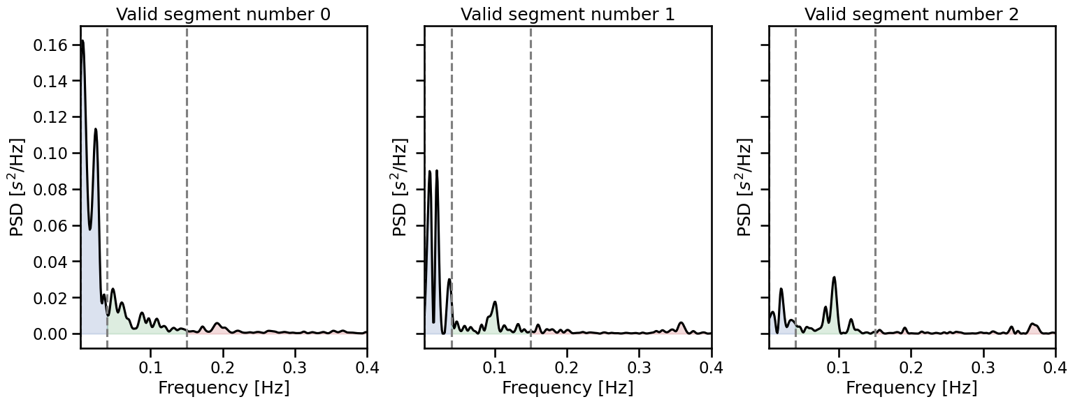
We can also provide the peaks vector directly and compute heart rate variability from the valid segments in this vector.
valids = get_valid_segments(signal=peaks, bad_segments=[(600000, 660000), (1000000, 1200000)])
_, axs = plt.subplots(1, 3, figsize=(18, 6), sharey=True)
for i, valid_peaks in enumerate(valids):
    plot_frequency(rr=valid_peaks, input_type="peaks", ax=axs[i])
    axs[i].set_title(f"Valid segment number {i}")