Instantaneous and evoked heart rate

Author: Nicolas Legrand nicolas.legrand@cfin.au.dk

Show code cell source Hide code cell source

%%capture
import sys
if 'google.colab' in sys.modules:
    ! pip install systole

import matplotlib.pyplot as plt
import seaborn as sns
import numpy as np
from systole.detection import ecg_peaks
from systole.plots import plot_rr, plot_evoked, plot_events
from systole import import_dataset1
from systole.utils import heart_rate, to_epochs

from bokeh.io import output_notebook
from bokeh.plotting import show
output_notebook()

sns.set_context('talk')

Loading BokehJS ...

This tutorial will cover instantaneous heart rate and evoked heart rate analysis. In the previous section, we analyzed the heart rate variability as a property that can be observed in longer cardiac recordings and that might reflect the influence of the sympathetic and/or the parasympathetic nervous system on behavior. This approach has been widely used in psychology and psychophysiology to evaluate the trait heart rate variability (HRV) of a given participant on a continuous domain, sometimes in conjunction with experimental manipulations. This approach requires relatively long recordings to give a reasonable estimate of the HRV (~5 minutes), and resting conditions are also required to let the nervous system returns to a baseline. In some cases, experimenters may want to also record and/or control for respiratory frequency as this has a known physiological impact on HRV, in particular in the lower frequency components.

However, psychophysiological interactions can appear at much shorter time scales (as fast as 1-2 seconds following stimulation), and these effects can be examined using evoked heart rate analysis. Evoked heart rate refers to the fluctuation of instantaneous heart rate following stimulation and could be described as the cardiac equivalent of event-related potentials ERP. These fast fluctuations in heart-rate have many sources, for example changes in noradrenaline and/or autonomic factors, emotional states, and other cognitive variables.

To perform evoked heart rate analysis, we need an ECG recording and a trigger, or stim channel, that will encode the occurrence of the events we want to study. Here, we will use an example dataset included in Systole. The task itself has been described in [Legrand et al., 2020]. During the recording, the participant has to rate the emotional valence of 36 neutral and 36 disgusting images (10 seconds max per image). The stim channel encodes the presentation of disgusting (2) and neutral (1) images.

# Import ECG recording and Stim channel
ecg_df = import_dataset1(modalities=['ECG', 'Stim'], disable=True)

Instantaneous heart rate

# Peak detection in the ECG signal using the Pan-Tompkins method
signal, peaks = ecg_peaks(signal=ecg_df.ecg, method='sleepecg', sfreq=1000)

Because the heartbeats are discrete events interleaved by unequal intervals, the instantaneous heart rate time series is the results of the interpolation of the individual heart rate estimates.

By defaults, the plot_rr function will linearly connect the dots to save memory.

show(
    plot_rr(peaks, input_type='peaks', backend='bokeh', figsize=250)
)

The heart_rate function provide more options and enables the user to select between different interpolation parameter following the ones povided by the scipy.interpolate.interpolate1d function.

# Select a subsample of the recording
this_peaks = peaks[20000:35000]

_, ax = plt.subplots(figsize=(13, 5))
for kind, color, style in zip(["cubic", "linear", "previous", "next"], 
                               sns.color_palette("deep", n_colors=4),
                               ["-", "--", ":", "-."]):
    hr, time = heart_rate(x=this_peaks, input_type='peaks', kind=kind)
    ax.plot(time, hr, color=color, label=kind, linestyle=style)

# Show individual heartbeats
ax.scatter(np.where(this_peaks)[0][1:]/1000,
           np.diff(np.where(this_peaks)[0]),
           s=100, color="gray", edgecolors="k", label="Heartbeats")
plt.legend()
ax.set_xlabel("Time (s)")
ax.set_ylabel("RR intervals (ms)")
ax.set_title("Interpolation of the instantaneous heart rate")
sns.despine()

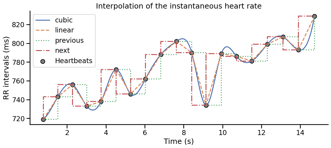
Note that here the timing of the peaks detection matters. The artefact correction, if it is used, should take this into account and never interpolate RR times series directly but always try to infer the presence, or absence, of cardiac cycles.

Evoked heart rate

Finding R peaks and extract instantaneous heart rate.

heartrate, new_time = heart_rate(peaks, kind='previous', unit='bpm')

Create stim vectors for neutral and discusting images separately. Here, 1 encode the presentation of an image.

triggers_idx = [
    np.where(ecg_df.stim.to_numpy() == 2)[0], 
    np.where(ecg_df.stim.to_numpy() == 1)[0]
]

neutral, disgust = np.zeros(len(new_time)), np.zeros(len(new_time))

disgust[np.round(np.where(ecg_df.stim.to_numpy() == 2)[0]).astype(int)] = 1
neutral[np.round(np.where(ecg_df.stim.to_numpy() == 1)[0]).astype(int)] = 1

Event plot

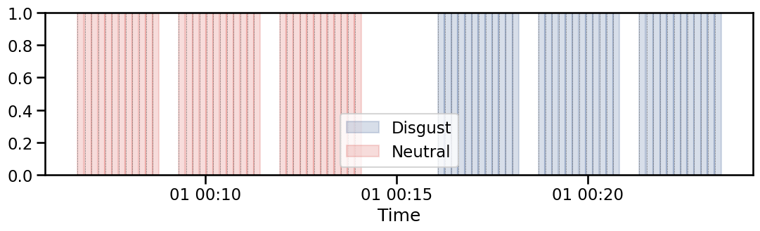
The plot_events function can be usefull to visualize the distribution of events during the task.

plot_events(triggers_idx=triggers_idx, backend="matplotlib", labels=["Disgust", "Neutral"],
            tmin=-0.5, tmax=10.0, palette=[sns.xkcd_rgb["denim blue"], sns.xkcd_rgb["pale red"]],
            figsize=(13, 3))

<Axes: xlabel='Time'>

This plot can be combined with other functionnalities of Systole, for example to wisualize the evolution of instantaneous heart rate across the different trials.

# First, we create a RR interval plot
show(
    plot_rr(
        peaks, input_type='peaks', backend='bokeh', figsize=250, 
        events_params={"triggers_idx": triggers_idx, "labels": ["Disgust", "Neutral"],
                       "tmin": -0.5, "tmax": 10.0, "palette": [sns.xkcd_rgb["denim blue"], sns.xkcd_rgb["pale red"]]}
    )
)

However, it is still difficult to see if a general tendency emerges from the time course of the heart rate following the stimulations, and if the two conditions differ from one another.

Evoked plot

Systole provides a function to_epochs that can easily convert raw signal and triggers vectors into the corresponding epochs array. An epoch is simply a 2d matrix containing the signal of interest sliced using some interval around the trigers. It is also common practice to baseline correct these signal using the value at t=0 or some interval before the stimuli (e.g., the average interval from 1 second pre-baseline), so the evoked response can be more readily interpreted.

This function accepts several arguments and can be used in a variety of ways (see documentation). Here, we provide the trigger idexes using the triggers_idx parameter (the sames where a trigger was recorded, here indicating that an image appeared on the screen). The apply_baseline parameter is set to (-1.0, 0.0) to indicate that we want substract the average of the signal value one second before the triggers appear.

epoch, rejected = to_epochs(signal=signal, triggers_idx=triggers_idx, apply_baseline=(-1.0, 0.0))

The function returns two objects:

• A 2d epoch array, that contains the signal of interest in the range around the trigger.

• A 1d reject array that indexes the rejected trials during the epoching process.

Trials can be rejected because

1. They contain artefacts. The artefacted part of the recording can be indexed using the reject parameter.

2. The time range of the trial lies outside the signal range. This can be the case for the first or the last trials

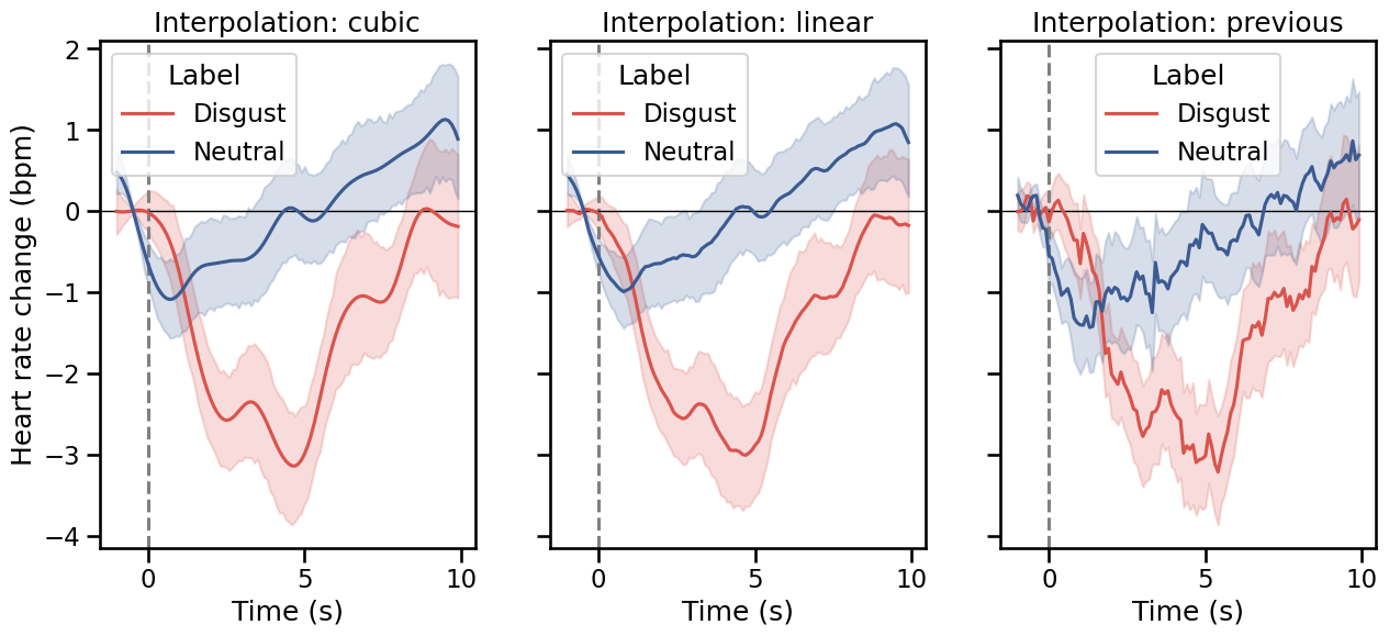
Visualization of the event related instantaneous heart rate:

show(
    plot_evoked(rr=peaks, triggers_idx=triggers_idx, input_type="peaks", backend="bokeh", 
                palette=[sns.xkcd_rgb["pale red"], sns.xkcd_rgb["denim blue"]], decim=100,
                apply_baseline=(-1.0, 0.0), figsize=(400, 400))
)

fig, axs = plt.subplots(1, 3, figsize=(15, 6), sharey=True)

for i, kind in enumerate(["cubic", "linear", "previous"]):
    axs[i].set_title(f"Interpolation: {kind}")
    plot_evoked(
        rr=peaks, triggers_idx=triggers_idx, input_type="peaks", kind=kind,
        palette=[sns.xkcd_rgb["pale red"], sns.xkcd_rgb["denim blue"]], labels=["Disgust", "Neutral"],
        decim=100, apply_baseline=(-1.0, 0.0), figsize=(6, 6), ax=axs[i], ci=68
    )

/opt/hostedtoolcache/Python/3.9.18/x64/lib/python3.9/site-packages/systole/plots/backends/matplotlib/plot_evoked.py:70: FutureWarning: 

The `ci` parameter is deprecated. Use `errorbar=('ci', 68)` for the same effect.

  sns.lineplot(data=epoch_df, x="Time", y="heart_rate", hue="Label", ax=ax, **kwargs)

/opt/hostedtoolcache/Python/3.9.18/x64/lib/python3.9/site-packages/systole/plots/backends/matplotlib/plot_evoked.py:70: FutureWarning: 

The `ci` parameter is deprecated. Use `errorbar=('ci', 68)` for the same effect.

  sns.lineplot(data=epoch_df, x="Time", y="heart_rate", hue="Label", ax=ax, **kwargs)

/opt/hostedtoolcache/Python/3.9.18/x64/lib/python3.9/site-packages/systole/plots/backends/matplotlib/plot_evoked.py:70: FutureWarning: 

The `ci` parameter is deprecated. Use `errorbar=('ci', 68)` for the same effect.

  sns.lineplot(data=epoch_df, x="Time", y="heart_rate", hue="Label", ax=ax, **kwargs)

This concludes the tutorial on using systole for evoked HR analysis!