Fitting single subject data using Bayesian estimation

Author: Nicolas Legrand nicolas.legrand@cfin.au.dk

%%capture
import sys
if 'google.colab' in sys.modules:
    ! pip install metadpy

import arviz as az
import numpy as np
from metadpy.bayesian import hmetad

From response-signal arrays

# Create responses data
nR_S1 = np.array([52, 32, 35, 37, 26, 12, 4, 2])
nR_S2 = np.array([2, 5, 15, 22, 33, 38, 40, 45])

This function will return two variable. The first one is a pymc model variable

model, traces = hmetad(nR_S1=nR_S1, nR_S2=nR_S2)

Auto-assigning NUTS sampler...

Initializing NUTS using jitter+adapt_diag...

Sequential sampling (4 chains in 1 job)

NUTS: [c1, d1, meta_d, cS1_hn, cS2_hn]

100.00% [2000/2000 00:18<00:00 Sampling chain 0, 0 divergences]

100.00% [2000/2000 00:18<00:00 Sampling chain 1, 0 divergences]

100.00% [2000/2000 00:17<00:00 Sampling chain 2, 0 divergences]

100.00% [2000/2000 00:18<00:00 Sampling chain 3, 0 divergences]

Sampling 4 chains for 1_000 tune and 1_000 draw iterations (4_000 + 4_000 draws total) took 73 seconds.

The rhat statistic is larger than 1.01 for some parameters. This indicates problems during sampling. See https://arxiv.org/abs/1903.08008 for details

The effective sample size per chain is smaller than 100 for some parameters.  A higher number is needed for reliable rhat and ess computation. See https://arxiv.org/abs/1903.08008 for details

az.plot_trace(traces, var_names=["c1", "d1", "meta_d", "cS1", "cS2"]);

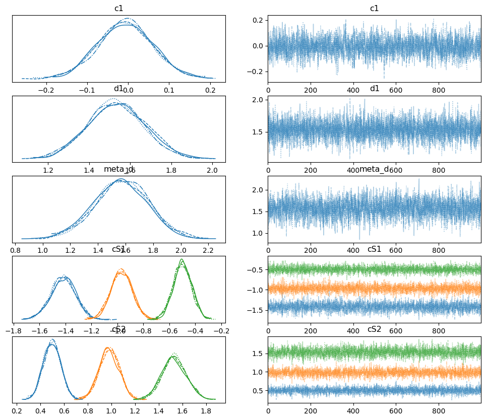
az.summary(traces, var_names=["c1", "d1", "meta_d", "cS1", "cS2"])

	mean	sd	hdi_3%	hdi_97%	mcse_mean	mcse_sd	ess_bulk	ess_tail	r_hat
c1	-0.007	0.067	-0.137	0.114	0.001	0.001	2435.0	2688.0	1.0
d1	1.532	0.139	1.279	1.801	0.002	0.001	4587.0	2882.0	1.0
meta_d	1.571	0.198	1.184	1.937	0.004	0.003	3027.0	3113.0	1.0
cS1[0]	-1.418	0.095	-1.595	-1.238	0.002	0.001	3154.0	3135.0	1.0
cS1[1]	-0.970	0.082	-1.123	-0.816	0.001	0.001	3284.0	3436.0	1.0
cS1[2]	-0.500	0.071	-0.626	-0.360	0.001	0.001	3970.0	3069.0	1.0
cS2[0]	0.499	0.073	0.368	0.636	0.001	0.001	4407.0	3227.0	1.0
cS2[1]	0.983	0.084	0.822	1.135	0.001	0.001	3294.0	3579.0	1.0
cS2[2]	1.531	0.102	1.345	1.729	0.002	0.001	3102.0	3345.0	1.0

Watermark

%load_ext watermark
%watermark -n -u -v -iv -w -p metadpy,pytensor,pymc

Last updated: Wed Nov 08 2023

Python implementation: CPython
Python version       : 3.9.18
IPython version      : 8.17.2

metadpy : 0.1.1
pytensor: 2.17.3
pymc    : 5.9.1

sys  : 3.9.18 (main, Aug 28 2023, 08:38:32) 
[GCC 11.4.0]
numpy: 1.25.2
arviz: 0.16.1

Watermark: 2.4.3