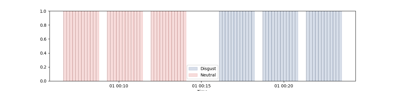
Plot events

import numpy as np
import seaborn as sns
from bokeh.io import output_notebook
from bokeh.plotting import show
from systole.detection import ecg_peaks
from systole.plots import plot_events, plot_rr

from systole import import_dataset1

# Author: Nicolas Legrand <nicolas.legrand@cfin.au.dk>
# Licence: GPL v3

Plot events distributions using Matplotlib as plotting backend

ecg_df = import_dataset1(modalities=['ECG', "Stim"])

# Get events triggers
triggers_idx = [
    np.where(ecg_df.stim.to_numpy() == 2)[0],
    np.where(ecg_df.stim.to_numpy() == 1)[0]
]

plot_events(
    triggers_idx=triggers_idx, labels=["Disgust", "Neutral"],
    tmin=-0.5, tmax=10.0, figsize=(13, 3),
    palette=[sns.xkcd_rgb["denim blue"], sns.xkcd_rgb["pale red"]],
)

  0%|          | 0/2 [00:00<?, ?it/s]
Downloading ECG channel:   0%|          | 0/2 [00:00<?, ?it/s]
Downloading ECG channel:  50%|█████     | 1/2 [00:00<00:00,  2.62it/s]
Downloading Stim channel:  50%|█████     | 1/2 [00:00<00:00,  2.62it/s]
Downloading Stim channel: 100%|██████████| 2/2 [00:00<00:00,  2.78it/s]
Downloading Stim channel: 100%|██████████| 2/2 [00:00<00:00,  2.75it/s]

<Axes: xlabel='Time'>

Plot events distributions using Bokeh as plotting backend and add the RR time series

output_notebook()

# Peak detection in the ECG signal using the Pan-Tompkins method
signal, peaks = ecg_peaks(ecg_df.ecg, method='pan-tompkins', sfreq=1000)

# First, we create a RR interval plot
rr_plot = plot_rr(peaks, input_type='peaks', backend='bokeh', figsize=250)

show(
    # Then we add events annotations to this plot using the plot_events function
    plot_events(triggers_idx=triggers_idx, backend="bokeh", labels=["Disgust", "Neutral"],
                tmin=-0.5, tmax=10.0, palette=[sns.xkcd_rgb["denim blue"], sns.xkcd_rgb["pale red"]],
                ax=rr_plot.children[0])
)