systole.plots.plot_ectopic

systole.plots.plot_ectopic(rr: None, artefacts: Dict[str, ndarray], input_type: str = 'rr_ms') → Union[figure, Axes]

systole.plots.plot_ectopic(rr: Union[List[float], ndarray], artefacts: None, input_type: str = 'rr_ms') → Union[figure, Axes]

systole.plots.plot_ectopic(rr: Union[List[float], ndarray], artefacts: Dict[str, ndarray], input_type: str = 'rr_ms') → Union[figure, Axes]

Visualization of ectopic beats detection.

The artefact detection is based on the method described in [1].

Parameters

rr

Interval time-series (R-R, beat-to-beat…), in miliseconds.

artefacts

The artefacts detected using systole.detection.rr_artefacts().

input_type

The type of input vector. Default is “rr_ms” for vectors of RR intervals, or interbeat intervals (IBI), expressed in milliseconds. Can also be “peaks” (a boolean vector where 1 represents the occurrence of R waves or systolic peaks) or “rr_s” for IBI expressed in seconds.

ax

Where to draw the plot. Default is None (create a new figure). Only applies when backend=”matplotlib”.

backend

Select plotting backend (“matplotlib” or “bokeh”. Defaults to “matplotlib”.

figsize

Figure size. Default is (13, 5) for Matplotlib backend, and the height is 600 when using Bokeh backend.

Returns

plot

The matplotlib axes, or the boken figure containing the plot.

See also

plot_shortlong, plot_subspaces

Notes

If both rr and artefacts are provided, the function will drop artefacts and re-evaluate given the current RR time-series.

References

1

Lipponen, J. A., & Tarvainen, M. P. (2019). A robust algorithm for heart rate variability time series artefact correction using novel beat classification. Journal of Medical Engineering & Technology, 43(3), 173–181. https://doi.org/10.1080/03091902.2019.1640306

Examples

Visualizing ectopic subspace from RR time series.

from systole import import_rr
from systole.plots import plot_ectopic

# Import PPG recording as numpy array
rr = import_rr().rr.to_numpy()

plot_ectopic(rr, input_type="rr_ms")

<Axes: title={'center': 'Subspace 1 \n (ectopic beats detection)'}, xlabel='Subspace $S_{11}$', ylabel='Subspace $S_{12}$'>

Visualizing ectopic subspace from the artefact dictionary generated by systole.detection.rr_artefacts().

from systole.detection import rr_artefacts

# Use the rr_artefacts function to find ectopic beats
artefacts = rr_artefacts(rr)

plot_ectopic(artefacts=artefacts)

<Axes: title={'center': 'Subspace 1 \n (ectopic beats detection)'}, xlabel='Subspace $S_{11}$', ylabel='Subspace $S_{12}$'>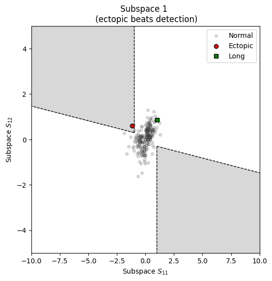

Using Bokeh as plotting backend.

from bokeh.io import output_notebook
from bokeh.plotting import show
from systole.detection import rr_artefacts
output_notebook()

# Use the rr_artefacts function to find ectopic beats
artefacts = rr_artefacts(rr)
show(
    plot_ectopic(artefacts=artefacts, backend="bokeh")
 )

Loading BokehJS ...