systole.plots.plot_subspaces

systole.plots.plot_subspaces(rr: Optional[Union[List[float], ndarray]] = None, artefacts: Optional[Dict[str, ndarray]] = None, input_type: str = 'rr_s', figsize: Optional[Union[Tuple[float, float], int]] = None, ax: Optional[Union[Tuple, List]] = None, backend: str = 'matplotlib') → Union[figure, Axes]

Visualization of short, long, extra, missed and ectopic beats detection.

The artefact detection is based on the method described in [1].

Parameters

rr

R-R interval time-series, peaks or peaks index vectors. The default expected vector is R-R intervals in milliseconds. Other data format can be provided by specifying the “input_type” (can be “rr_s”, “peaks” or “peaks_idx”).

artefacts

A dictionary containing the infos abount the artefacts detected using the systole.detection.rr_artefacts() function. This parameter is optional, but if provided the data provided in rr will be ignored.

input_type

The type of input vector. Default is “peaks” (a boolean vector where 1 represents the occurrence of R waves or systolic peaks). Can also be “rr_s” or “rr_ms” for vectors of RR intervals, or interbeat intervals (IBI), expressed in seconds or milliseconds (respectively).

figsize

Figure size. Default is (12, 6) for matplotlib backend, and the height is 600 when using bokeh backend.

ax

Where to draw the plot. Default is None (create a new figure). Otherwise, a tuple of list of Matplotlib axes should be provided. Only applies if backend=”matplotlib”.

backend

Select plotting backend {“matplotlib”, “bokeh”}. Defaults to “matplotlib”.

Returns

plot

The matplotlib axes, or the boken figure containing the plot.

See also

plot_events, plot_ectopic, plot_shortlong, plot_subspaces, plot_frequency

plot_timedomain, plot_nonlinear

References

1

Lipponen, J. A., & Tarvainen, M. P. (2019). A robust algorithm for heart rate variability time series artefact correction using novel beat classification. Journal of Medical Engineering & Technology, 43(3), 173–181. https://doi.org/10.1080/03091902.2019.1640306

Examples

Visualizing artefacts from RR time series.

from systole import import_rr
from systole.plots import plot_subspaces
import matplotlib.pyplot as plt

# Import PPG recording as numpy array
rr = import_rr().rr.to_numpy()

_, axs = plt.subplots(ncols=2, figsize=(12, 6))
plot_subspaces(rr, ax=axs)

(<Axes: title={'center': 'Subspace 1 \n (ectopic beats detection)'}, xlabel='Subspace $S_{11}$', ylabel='Subspace $S_{12}$'>,
 <Axes: title={'center': 'Subspace 2 \n (long and short beats detection)'}, xlabel='Subspace $S_{21}$', ylabel='Subspace $S_{22}$'>)

Visualizing artefacts from the artefact dictionary.

from systole.detection import rr_artefacts

# Use the rr_artefacts function to short/long and extra/missed intervals
artefacts = rr_artefacts(rr)

_, axs = plt.subplots(ncols=2, figsize=(12, 6))
plot_subspaces(artefacts=artefacts, ax=axs)

(<Axes: title={'center': 'Subspace 1 \n (ectopic beats detection)'}, xlabel='Subspace $S_{11}$', ylabel='Subspace $S_{12}$'>,
 <Axes: title={'center': 'Subspace 2 \n (long and short beats detection)'}, xlabel='Subspace $S_{21}$', ylabel='Subspace $S_{22}$'>)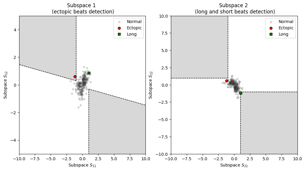

Using Bokeh as plotting backend.

from bokeh.io import output_notebook
from bokeh.plotting import show
from systole.detection import rr_artefacts
output_notebook()

show(
   plot_subspaces(
     artefacts=artefacts, backend="bokeh", figsize=400
     )
)

Loading BokehJS ...